Configuration Footprint
This plugin helps you explore how thoroughly the optimizer has explored your configuration space and view its preferences during the run.
This plugin is capable of answering following questions:
Was the configuration space well-covered by the optimizer?
Can I stop the optimization process or should I invest more computational resources?
Which hyperparameter values are considered favorable?
First, let’s briefly mention the various kinds of configurations we are concerned with here:
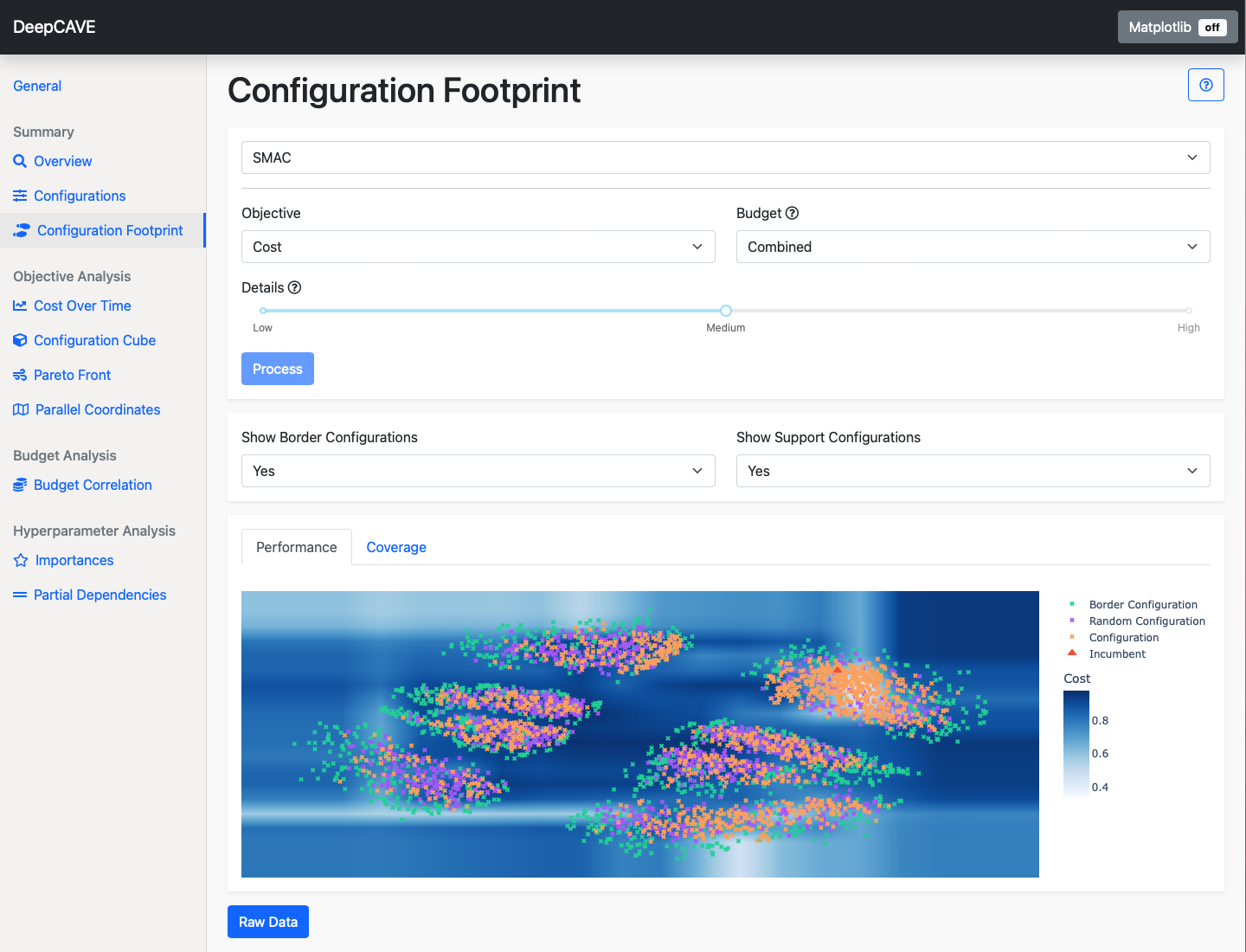
Incumbent: The best configuration identified for a given objective, like cost or time, shown as a red triangle.
Evaluated Configurations: Configurations that have been assessed by the optimizer, with known true objective values, marked with orange x’s.
Random Configurations: Configurations that have been sampled randomly from the configuration space, indicated by purple x’s.
Border Configurations: Configurations located at the edges of the configuration space, corresponding to the minimum and maximum values for scalar parameters, shown as green x’s.
By leveraging the evaluated configurations and the incumbent for each objective and budget, we gain insights into the expected objective values around these points and can infer information about other points in the configuration space.
To visualize a high-dimensional configuration space in 2D, we use a dimensionality reduction algorithm, here MDS. MDS aims to preserve distances as accurately as possible when mapping from a high-dimensional space to a lower-dimensional one. While not perfect, this technique provides valuable insights.
There are two plots available. Both share the same axes, with points plotted in consistent coordinates. Switching between them will provide a comprehensive understanding of your configuration footprint:
Performance plot
The performance plot is particularly useful for understanding which configurations are likely to achieve specific objective scores. By hovering over the incumbent, you can identify the best configuration found for the given objective and budget.
Note
For non-deterministic runs (where multiple seeds are evaluated per configuration), only configurations evaluated with the maximum number of seeds are considered for determining the best configuration.
The evaluated configurations have actual objective scores, though these may be noisy if the objective itself is noisy. By leveraging a surrogate model, we can use them to approximate the performance of other areas in the configuration space. This approximation is represented by the background colour. It does not reflect the true objective value in areas where no configurations have been evaluated.
To improve resolution, you can use the Details option, which adjusts the grid size for the plot. Note that increasing resolution will also increase computation time.
Coverage plot
The coverage plot provides an overview of how well your configuration space has been sampled and highlights which regions have been most thoroughly evaluated. Border configurations are particularly informative here, showing the edges of the 2D representation of your configuration space. There will likely be small clusters of evaluated points, where the optimizer focused on finding optimal configurations, as well as scattered points across valid regions to provide a broad understanding of scores for various objectives.
Options
Objective: Select the objective function you wish to analyze.
Budget: Select the multi-fidelity budget to be used. The plugin will only consider trials evaluated on the selected budget. The Combined budget option displays all configurations but shows scores only from the highest budget if a configuration was evaluated with multiple budgets.
Details: Controls the resolution of the surface plot.
To refine your analysis, you can apply various filters after calculation:
Show Border Configurations: Whether to display border configurations.
Show Support Configurations: Whether to display random configurations.