Visualizing the Results

Auto-Pytorch uses SMAC to fit individual machine learning algorithms and then ensembles them together using Ensemble Selection.

The following examples shows how to visualize both the performance of the individual models and their respective ensemble.

Additionally, as we are compatible with scikit-learn, we show how to further interact with Scikit-Learn Inspection support.

import os
import pickle
import tempfile as tmp
import time
import warnings

# The following variables are not needed for every unix distribution, but are
# highlighted in here to prevent problems with multiprocessing with scikit-learn.
os.environ['JOBLIB_TEMP_FOLDER'] = tmp.gettempdir()
os.environ['OMP_NUM_THREADS'] = '1'
os.environ['OPENBLAS_NUM_THREADS'] = '1'
os.environ['MKL_NUM_THREADS'] = '1'

warnings.simplefilter(action='ignore', category=UserWarning)
warnings.simplefilter(action='ignore', category=FutureWarning)

import matplotlib.pyplot as plt

import numpy as np

import pandas as pd


import sklearn.datasets
import sklearn.model_selection
from sklearn.inspection import permutation_importance

from smac.tae import StatusType


from autoPyTorch.api.tabular_classification import TabularClassificationTask
from autoPyTorch.metrics import accuracy

Data Loading

# We will use the iris dataset for this Toy example
seed = 42
X, y = sklearn.datasets.fetch_openml(data_id=61, return_X_y=True, as_frame=True)
X_train, X_test, y_train, y_test = sklearn.model_selection.train_test_split(
    X,
    y,
    random_state=42,
)

Build and fit a classifier

api = TabularClassificationTask(seed=seed)
api.search(
    X_train=X_train,
    y_train=y_train,
    X_test=X_test.copy(),
    y_test=y_test.copy(),
    optimize_metric=accuracy.name,
    total_walltime_limit=200,
    func_eval_time_limit_secs=50
)

<autoPyTorch.api.tabular_classification.TabularClassificationTask object at 0x7f9a9f425f10>

One can also save the model for future inference

# For more details on how to deploy a model, please check
# `Scikit-Learn persistence
# <https://scikit-learn.org/stable/modules/model_persistence.html>`_ support.
with open('estimator.pickle', 'wb') as handle:
    pickle.dump(api, handle, protocol=pickle.HIGHEST_PROTOCOL)

# Then let us read it back and use it for our analysis
with open('estimator.pickle', 'rb') as handle:
    estimator = pickle.load(handle)

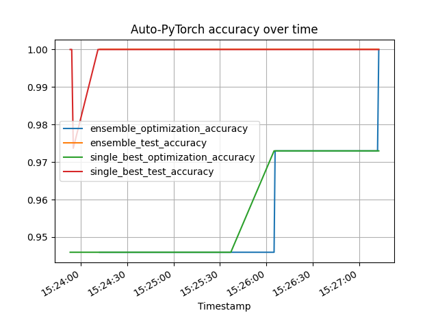
Plotting the model performance

# We will plot the search incumbent through time.

# Collect the performance of individual machine learning algorithms
# found by SMAC
individual_performances = []
for run_key, run_value in estimator.run_history.data.items():
    if run_value.status != StatusType.SUCCESS:
        # Ignore crashed runs
        continue
    individual_performances.append({
        'Timestamp': pd.Timestamp(
            time.strftime(
                '%Y-%m-%d %H:%M:%S',
                time.localtime(run_value.endtime)
            )
        ),
        'single_best_optimization_accuracy': accuracy._optimum - run_value.cost,
        'single_best_test_accuracy': np.nan if run_value.additional_info is None else
        accuracy._optimum - run_value.additional_info['test_loss']['accuracy'],
    })
individual_performance_frame = pd.DataFrame(individual_performances)

# Collect the performance of the ensemble through time
# This ensemble is built from the machine learning algorithms
# found by SMAC
ensemble_performance_frame = pd.DataFrame(estimator.ensemble_performance_history)

# As we are tracking the incumbent, we are interested in the cummax() performance
ensemble_performance_frame['ensemble_optimization_accuracy'] = ensemble_performance_frame[
    'train_accuracy'
].cummax()
ensemble_performance_frame['ensemble_test_accuracy'] = ensemble_performance_frame[
    'test_accuracy'
].cummax()
ensemble_performance_frame.drop(columns=['test_accuracy', 'train_accuracy'], inplace=True)
individual_performance_frame['single_best_optimization_accuracy'] = individual_performance_frame[
    'single_best_optimization_accuracy'
].cummax()
individual_performance_frame['single_best_test_accuracy'] = individual_performance_frame[
    'single_best_test_accuracy'
].cummax()

pd.merge(
    ensemble_performance_frame,
    individual_performance_frame,
    on="Timestamp", how='outer'
).sort_values('Timestamp').fillna(method='ffill').plot(
    x='Timestamp',
    kind='line',
    legend=True,
    title='Auto-PyTorch accuracy over time',
    grid=True,
)
plt.show()