Model Explanation

The following example shows how to fit a simple classification model with auto-sklearn and use the inspect module from scikit-learn to understand what affects the predictions.

import sklearn.datasets
from sklearn.inspection import plot_partial_dependence, permutation_importance
import matplotlib.pyplot as plt
import autosklearn.classification

Load Data and Build a Model

We start by loading the “Run or walk” dataset from OpenML and train an auto-sklearn model on it. For this dataset, the goal is to predict whether a person is running or walking based on accelerometer and gyroscope data collected by a phone. For more information see here.

dataset = sklearn.datasets.fetch_openml(data_id=40922)

# Note: To speed up the example, we subsample the dataset
dataset.data = dataset.data.sample(n=5000, random_state=1, axis="index")
dataset.target = dataset.target[dataset.data.index]

X_train, X_test, y_train, y_test = sklearn.model_selection.train_test_split(
    dataset.data, dataset.target, test_size=0.3, random_state=1
)

automl = autosklearn.classification.AutoSklearnClassifier(
    time_left_for_this_task=120,
    per_run_time_limit=30,
    tmp_folder="/tmp/autosklearn_inspect_predictions_example_tmp",
)
automl.fit(X_train, y_train, dataset_name="Run_or_walk_information")

s = automl.score(X_train, y_train)
print(f"Train score {s}")
s = automl.score(X_test, y_test)
print(f"Test score {s}")

/home/runner/work/auto-sklearn/auto-sklearn/autosklearn/data/target_validator.py:187: UserWarning: Fitting transformer with a pandas series which has the dtype category. Inverse transform may not be able preserve dtype when converting to np.ndarray
  warnings.warn(
Train score 0.9948571428571429
Test score 0.9813333333333333

Compute permutation importance - part 1

Since auto-sklearn implements the scikit-learn interface, it can be used with the scikit-learn’s inspection module. So, now we first look at the permutation importance, which defines the decrease in a model score when a given feature is randomly permuted. So, the higher the score, the more does the model’s predictions depend on this feature.

Note: There are some pitfalls in interpreting these numbers, which can be found in the scikit-learn docs.

r = permutation_importance(automl, X_test, y_test, n_repeats=10, random_state=0)
sort_idx = r.importances_mean.argsort()[::-1]

plt.boxplot(
    r.importances[sort_idx].T, labels=[dataset.feature_names[i] for i in sort_idx]
)

plt.xticks(rotation=90)
plt.tight_layout()
plt.show()

for i in sort_idx[::-1]:
    print(
        f"{dataset.feature_names[i]:10s}: {r.importances_mean[i]:.3f} +/- "
        f"{r.importances_std[i]:.3f}"
    )

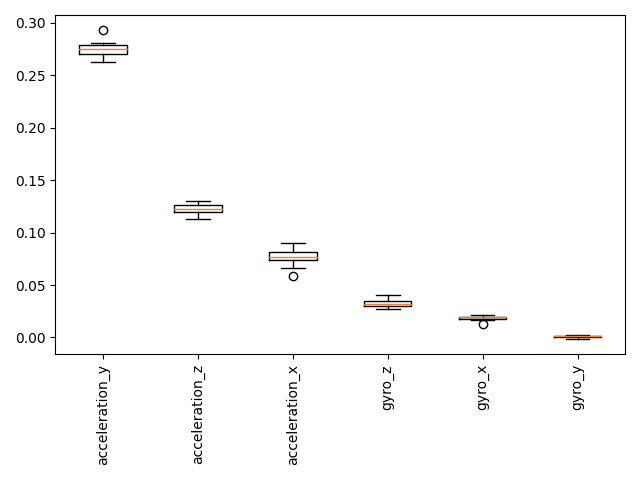
gyro_y    : 0.001 +/- 0.001
gyro_x    : 0.018 +/- 0.002
gyro_z    : 0.033 +/- 0.004
acceleration_x: 0.076 +/- 0.009
acceleration_z: 0.123 +/- 0.005
acceleration_y: 0.275 +/- 0.008

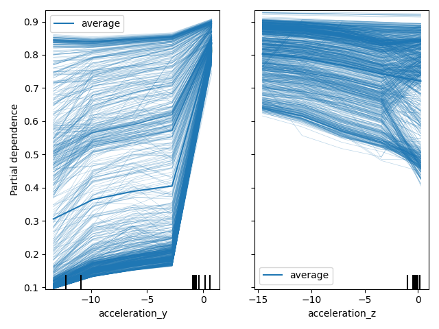
Create partial dependence (PD) and individual conditional expectation (ICE) plots - part 2

ICE plots describe the relation between feature values and the response value for each sample individually – it shows how the response value changes if the value of one feature is changed.

PD plots describe the relation between feature values and the response value, i.e. the expected response value wrt. one or multiple input features. Since we use a classification dataset, this corresponds to the predicted class probability.

Since acceleration_y and acceleration_z turned out to have the largest impact on the response value according to the permutation dependence, we’ll first look at them and generate a plot combining ICE (thin lines) and PD (thick line)

features = [1, 2]
plot_partial_dependence(
    automl,
    dataset.data,
    features=features,
    grid_resolution=5,
    kind="both",
    feature_names=dataset.feature_names,
)
plt.tight_layout()
plt.show()

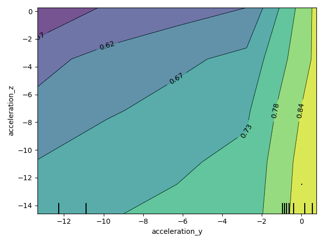
Create partial dependence (PDP) plots for more than one feature - part 3

A PD plot can also be generated for two features and thus allow to inspect the interaction between these features. Again, we’ll look at acceleration_y and acceleration_z.

features = [[1, 2]]
plot_partial_dependence(
    automl,
    dataset.data,
    features=features,
    grid_resolution=5,
    feature_names=dataset.feature_names,
)
plt.tight_layout()
plt.show()